PyTorch and Zounds
In a previous post, we used zounds to build a very simple synthesizer by learning K-Means centroids from individual frames of a spectrogram, and then using the sequence of one-hot encodings as parameters for our synthesizer.
Recently, zounds has added support for training and employing PyTorch models, and I wanted to try out something similar using a trained autoencoder, rather than K-Means clustering.
There’s been a ton of research and interest lately around using deep neural networks for audio synthesis (e.g. WaveNet and NSynth), and while this post describes a very simple, “toy” approach to the problem, it illustrates how zounds can be used for all kinds of interesting machine-learning experiments dealing with audio.
As usual, if you want to jump ahead, you can see the entire example here.
Extracing Features from a Dataset
First, we’ll need to extract the features that the autoencoder will be trained on. In this example, we’re going to diverge from our previous K-Means example in a couple ways:
- First, we’ll learn from a little over half a second of audio at a time, rather than learning codes from a single MDCT frame, which only has a duration of tens of milliseconds
- Second, the spectrograms we learn from will use a geometric, rather than a linear scale, so that the model our autoencoder tries to compress more closely matches human pitch perception
Defining the Graph
With further ado, here’s our processing graph:
samplerate = zounds.SR11025()
BaseModel = zounds.stft(resample_to=samplerate, store_fft=True)

scale = zounds.GeometricScale(
    start_center_hz=300,
    stop_center_hz=3040,
    bandwidth_ratio=0.016985,
    n_bands=300)
scale.ensure_overlap_ratio(0.5)


@zounds.simple_lmdb_settings('sounds', map_size=1e10, user_supplied_id=True)
class Sound(BaseModel):
    """
    An audio processing pipeline that computes a frequency domain representation
    of the sound that follows a geometric scale
    """
    bark = zounds.ArrayWithUnitsFeature(
        zounds.BarkBands,
        samplerate=samplerate,
        stop_freq_hz=samplerate.nyquist,
        needs=BaseModel.fft,
        store=True)

    long_windowed = zounds.ArrayWithUnitsFeature(
        zounds.SlidingWindow,
        wscheme=zounds.SampleRate(
            frequency=zounds.Milliseconds(340),
            duration=zounds.Milliseconds(680)),
        wfunc=zounds.OggVorbisWindowingFunc(),
        needs=BaseModel.resampled,
        store=True)

    long_fft = zounds.ArrayWithUnitsFeature(
        zounds.FFT,
        needs=long_windowed,
        store=True)

    freq_adaptive = zounds.FrequencyAdaptiveFeature(
        zounds.FrequencyAdaptiveTransform,
        transform=np.fft.irfft,
        scale=scale,
        window_func=np.hanning,
        needs=long_fft,
        store=False)

    encoded = zounds.ArrayWithUnitsFeature(
        zounds.Learned,
        learned=FreqAdaptiveAutoEncoder(),
        needs=freq_adaptive,
        store=False)
Frequency-Adaptive Features
This model takes an approach inspired by the following papers:
- A quasi-orthogonal, invertible, and perceptually relevant time-frequency transform for audio coding
- A FRAMEWORK FOR INVERTIBLE, REAL-TIME CONSTANT-Q TRANSFORMS
Instead of computing an FFT over very short windows (tens of milliseconds) of overlapping audio frames, and ending up with a linear frequency scale, we instead:
- compute the FFT over much longer (hundreds of milliseconds) windows
- compute the inverse FFT of coefficients from the previous step, using windows of coefficients that vary in size, increasing as you move from low to high frequencies
Downloading and Processing the Data
Zounds has a datasets module
that defines classes for pulling data from some good sources for free audio on
the internet. For this example, we’ll extract features from these Bach pieces
hosted by the amazing Internet Archive.
The example code uses argparse
to accept an arbitrary Internet Archive id, which defaults to the Bach pieces
mentioned above.
parser = argparse.ArgumentParser()
parser.add_argument(
    '--internet-archive-id',
    help='the internet archive id to process',
    type=str,
    required=False,
    default='AOC11B')
args = parser.parse_args()

zounds.ingest(
    dataset=zounds.InternetArchive(args.internet_archive_id),
    cls=Sound,
    multi_threaded=True)
Learning the AutoEncoder Model
At this point, we’ve extracted and stored our frequency-adaptive representations for all of the Bach pieces, and now we’d like to train an autoencoder to produce a “compressed” representation of this representation, exploiting the structure and correlations in the data.
Getting a Feel for our Feature
First, let’s get a feel ourselves for what an individual training example looks like. Since the number of samples for a given time window actually varies by frequency band, it’s a little tough to visualize our feature, so we’ll cheat just a little:
>>> snds = list(Sound)
>>> snd = random.choice(snds)
>>> zounds.mu_law(snd.freq_adaptive.rasterize(64)[3])
Note that we’re:
- calling
zounds.mu_lawso that the magnitude of the coefficients holds more closely to human loudness perception (i.e., we perceive loudness on roughly a logarithmic, as opposed to linear, scale) - calling
snd.freq_adaptive.rasterize, which resamples each frequency band so that they contain the same number of samples for a given time window, making it possible to display the representation as an image.
Defining the Learning Pipeline
Similar to our ad-hoc code example above, we’ll want our learning pipeline to pre-process the data in a couple of different ways, so that our autoencoder optimizes for reproducing things that are perceptually salient to us humans.
Our pipeline will:
- Use mu-law companding so that the autoencoder is presented with magnitudes on a roughly logarithmic scale
- Scale each instance to have a maximum absolute value of one, again, since we primarily care about the shape of the data (i.e., the relationships of coefficients within a particular example).
@zounds.simple_settings
class FreqAdaptiveAutoEncoder(ff.BaseModel):
    """
    Define a processing pipeline to learn a compressed representation of the
    Sound.freq_adaptive feature.  Once this is trained and the pipeline is
    stored, we can apply all the pre-processing steps and the autoencoder
    forward and in reverse.
    """
    docs = ff.Feature(ff.IteratorNode)

    shuffle = ff.PickleFeature(
        zounds.ShuffledSamples,
        nsamples=500000,
        dtype=np.float32,
        needs=docs)

    mu_law = ff.PickleFeature(
        zounds.MuLawCompressed,
        needs=shuffle)

    scaled = ff.PickleFeature(
        zounds.InstanceScaling,
        needs=mu_law)

    autoencoder = ff.PickleFeature(
        zounds.PyTorchAutoEncoder,
        trainer=zounds.SupervisedTrainer(
            AutoEncoder(),
            loss=nn.MSELoss(),
            optimizer=lambda model: optim.Adam(model.parameters(), lr=0.00005),
            epochs=100,
            batch_size=64,
            holdout_percent=0.5),
        needs=scaled)

    # assemble the previous steps into a re-usable pipeline, which can perform
    # forward and backward transformations
    pipeline = ff.PickleFeature(
        zounds.PreprocessingPipeline,
        needs=(mu_law, scaled, autoencoder),
        store=True)
You can see from the example above that this processing graph has a pipeline
leaf that will compose mu_law, scaled, and autoencoder into a single
function that can be run forward and backward (more on this in just a bit).
And here’s how we’ve defined our PyTorch autoencoder:
class Layer(nn.Module):
    """
    A single layer of our simple autoencoder
    """

    def __init__(self, in_size, out_size):
        super(Layer, self).__init__()
        self.linear = nn.Linear(in_size, out_size, bias=False)
        self.tanh = nn.Tanh()

    def forward(self, inp):
        x = self.linear(inp)
        x = self.tanh(x)
        return x


class AutoEncoder(nn.Module):
    """
    A simple autoencoder.  No bells, whistles, or convolutions
    """

    def __init__(self):
        super(AutoEncoder, self).__init__()
        self.encoder = nn.Sequential(
            Layer(8192, 1024),
            Layer(1024, 512),
            Layer(512, 256))
        self.decoder = nn.Sequential(
            Layer(256, 512),
            Layer(512, 1024),
            Layer(1024, 8192))

    def forward(self, inp):
        encoded = self.encoder(inp)
        decoded = self.decoder(encoded)
        return decoded
Learning the Model
Now, it’s time to sample from our stored features, and let the autoencoder spend
some time training. Taking a look once more at the autoencoder node in our
graph…
autoencoder = ff.PickleFeature(
    zounds.PyTorchAutoEncoder,
    trainer=zounds.SupervisedTrainer(
        AutoEncoder(),
        loss=nn.MSELoss(),
        optimizer=lambda model: optim.Adam(model.parameters(), lr=0.00005),
        epochs=100,
        batch_size=64,
        holdout_percent=0.5),
    needs=scaled)
…we can see that we’ll use mean squared error as our loss function, Adam as our optimizer, training for 100 epochs (full passes over the data). We’ll hold out 50% of the samples for our test set, to ensure that we’re not overfitting the data (i.e., failing to generalize).
To initiate training, we run the following code:
if not FeatureTransfer.exists():
    FeatureTransfer.process(
        docs=(dict(data=doc.rasterized, labels=doc.freq_adaptive)
              for doc in Sound))
Evaluating the Model (Subjectively)
Once the model is trained, we can get a sense of how well it learned to compress an 8192-dimensional vector into only 256 features.
Let’s choose a Bach piece at random, and run the model both forward and backward to see how our reconstruction sounds:
# get a reference to the trained pipeline
autoencoder = FreqAdaptiveAutoEncoder()

# get references to all the sounds.  features are lazily
# loaded/evaluated, so this is a cheap operation
snds = list(Sound)

# create a synthesizer that can invert the frequency adaptive representation
synth = zounds.FrequencyAdaptiveFFTSynthesizer(scale, samplerate)


def random_reconstruction(random_encoding=False):
    # choose a random sound
    snd = choice(snds)

    # run the model forward
    encoded = autoencoder.pipeline.transform(snd.freq_adaptive)

    if random_encoding:
        mean = encoded.data.mean()
        std = encoded.data.std()
        encoded.data = np.random.normal(mean, std, encoded.data.shape)

    # then invert the encoded version
    inverted = encoded.inverse_transform()

    # compare the audio of the original and the reconstruction
    original = synth.synthesize(snd.freq_adaptive)
    recon = synth.synthesize(inverted)
    return original, recon, encoded.data, snd.freq_adaptive, inverted


# get the original audio, and the reconstructed audio
orig_audio, recon_audio, encoded, orig_coeffs, inverted_coeffs = \
    random_reconstruction()
Here’s the original Bach piece:
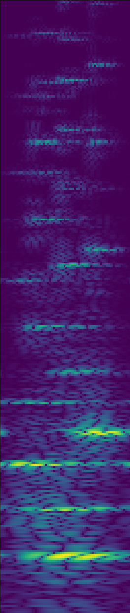
And here’s what the original (rasterized) coefficients look like:
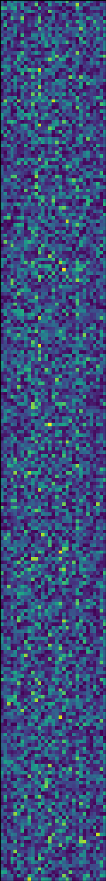
Here’s a subset of the encoded (256-dimensional) representation. What’s neat is
that the encoded representation is still an ArrayWithUnits instance, and can
thus be indexed into using a TimeSlice (as well as vanilla integer indices):
>>> encoded[zounds.TimeSlice(start=zounds.Seconds(1), duration=zounds.Seconds(2)]
Finally, it’s the moment we’ve all been waiting for! What does the reconstruction sound like?
The quality ain’t great, but there’s no question that our autoencoder has learned something about the structure of the original representation.
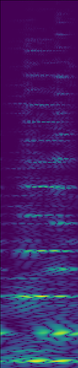
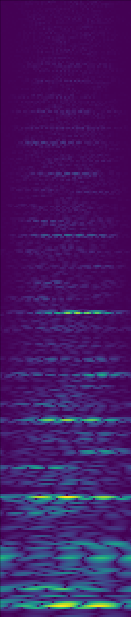
Here’s what the reconstructed (rasterized) coefficients look like:
Producing Novel Sounds?
What if we produce random encodings, and run the model backward? If we were to do this with raw audio samples, or even frequency-domain coefficients, we’d end up with white noise.
While it isn’t beautiful (or even necessarily pleasant) to listen to, you can understand the structure our model has learned (and the assumptions it makes) by doing the following:
>>> orig_audio, recon_audio, encoded, orig_coeffs, inverted_coeffs = \
random_reconstruction(random_encoding=True)
Note that this will produce noise in normal distribution that matches the mean and standard deviation of the encoding from a real Bach piece.
It sounds like someone banging on a piano!