Building a Simple Audio Encoder
Previously, we covered extracting some commonly used features from audio, and building a search. In this post, we’ll use a similar workflow to build a very rudimentary audio encoder and decoder. If you want to jump ahead, the complete code for this example is here.
The Modified Discrete Cosine Transform
We’ll be using the mofified discrete cosine transform (or MDCT for short), as the basis for our encoder. The Ogg Vorbis audio encoding also takes the MDCT as its starting point
A cosine transform uses a set of cosine functions, oscillating at different frequencies, as its basis functions, and expresses a time-domain signal as a linear combination of these frequencies.
To get an idea of what’s happening here, we can fire up zounds’ interactive, in-browser REPL and run the following:
>>> synth = zounds.SineSynthesizer(zounds.SR22050())
>>> signal = zounds.synthesize(zounds.Seconds(1), freqs_in_hz=[440., 660., 880.])
>>> from scipy.fftpack import dct
>>> dct(signal)
This will display an image where you can clearly see that the three sine waves we created are now represented as large coefficients for the cosine basis functions at those frequencies.
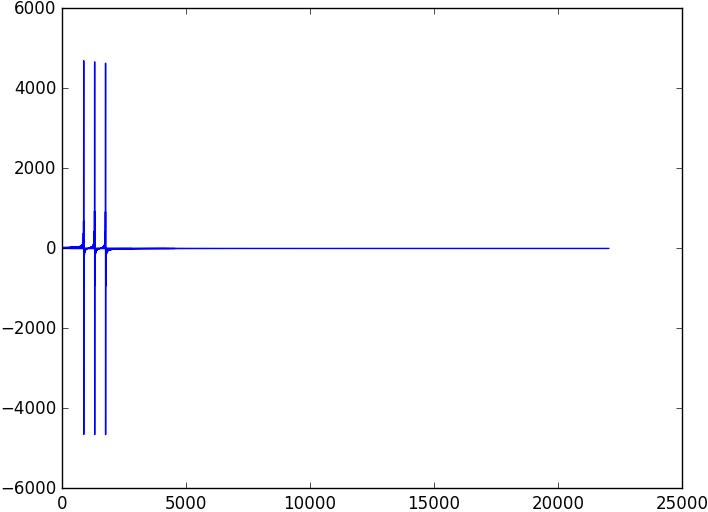
While we can perfectly reconstruct the original signal given these coefficients , we have poor localization in time. The MDCT solves this problem by applying the same transformation to short, overlapping blocks of a signal.
If we use the processing graph like this…
import featureflow as ff
import zounds
from random import choice

samplerate = zounds.SR11025()
STFT = zounds.stft(resample_to=samplerate)


class Settings(ff.PersistenceSettings):
    """
    These settings make it possible to specify an id (rather than automatically
    generating one) when analyzing a file, so that it's easier to reference
    that file by name later.
    """
    id_provider = ff.UserSpecifiedIdProvider(key='_id')
    key_builder = ff.StringDelimitedKeyBuilder()
    database = ff.LmdbDatabase(
            'mdct_synth', map_size=1e10, key_builder=key_builder)


class Document(STFT, Settings):
    """
    Inherit from a basic processing graph, and add a Modified Discrete Cosine
    Transform feature
    """
    mdct = zounds.TimeFrequencyRepresentationFeature(
            zounds.MDCT,
            needs=STFT.windowed,
            store=True)
…to extract the MDCT instead, we end up with something a bit more useful. Running…
>>> _id = Document.process(meta=signal.encode())
>>> doc = Document(_id)
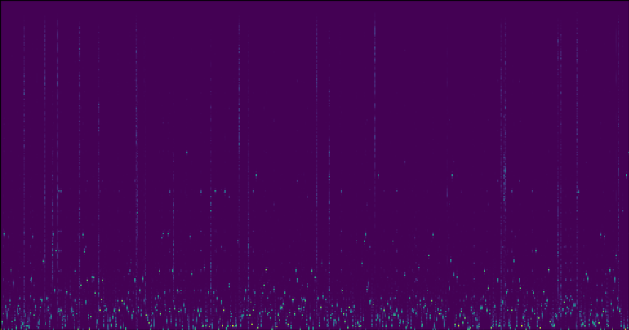
>>> doc.mdct[:, :100] # only look at lower frequencies, for brevity
will display something like this:

Here, you can see the same peaks, but instead of a single vector representing coefficients for the entire signal, we see a vector of coefficients (frequency is along the y-axis) for each short slice of time (time is along the x-axis).
We can recover the original audio by doing the following:
>>> mdct_synth = zounds.MDCTSynthesizer()
>>> mdct_synth.synthesize(doc.mdct)
The above code will:
- multiply the MDCT coefficients in each frameby the cosine basis functions, turning the frequency-domain representation back into a time-domain one
- Apply a windowing function to the time-domain frames to avoid artifacts at block boundaries
- Add the overlapping frames back together, resulting in a continuous, time-domain signal that can be streamed directly to an audio device
The Encoding Idea
Cosines osciallating at different frequencies serve as good basis functions, and allow us to express pretty much any sound imaginable, but on their own, they don’t allow us to compress the audio much, which is one very desirable feature of an audio encoding.
Pure tones don’t occur much in natural sounds; nature is full of transients (broad-spectrum noise that doesn’t last long), and vibrating physical bodies that produce rich harmonics (think lots of octaves, thirds and fifths on top of the fundamental).
If we choose basis functions that take advantage of the fact that certain spectral shapes are seen (or rather heard) frequently in the real world, it’s possible that we can get a decent compression ratio, and perhaps even an interpretable encoding.
Simple K-Means Clustering
One incredibly straightforward way to learn basis functions from real-world data is k-means clustering, which in our case, will learn K basis functions corresponding to commonly occurring spectral shapes from our training data. For example, there might be a cluster or centroid corresponding to the broad-band noise of a snare attack, and another centroid corresponding to the fundamental frequency and harmonics produced by human vocal cords.
We can define the following graph…
@zounds.simple_settings
class DctKmeans(ff.BaseModel):
    """
    A pipeline that does example-wise normalization by giving each example
    unit-norm, and learns 512 centroids from those examples.
    """
    docs = ff.Feature(
            ff.IteratorNode,
            store=False)

    # randomize the order of the data
    shuffle = ff.NumpyFeature(
            zounds.ReservoirSampler,
            nsamples=1e6,
            needs=docs,
            store=True)

    # give each frame unit norm, since we care about the shape of the spectrum
    # and not its magnitude
    unit_norm = ff.PickleFeature(
            zounds.UnitNorm,
            needs=shuffle,
            store=False)

    # learn 512 centroids, or basis functions
    kmeans = ff.PickleFeature(
            zounds.KMeans,
            centroids=512,
            needs=unit_norm,
            store=False)

    # assemble the previous steps into a re-usable pipeline, which can perform
    # forward and backward transformations
    pipeline = ff.PickleFeature(
            zounds.PreprocessingPipeline,
            needs=(unit_norm, kmeans),
            store=True)
…and learn the centroids:
DctKmeans.process(docs=(doc.mdct for doc in Document))
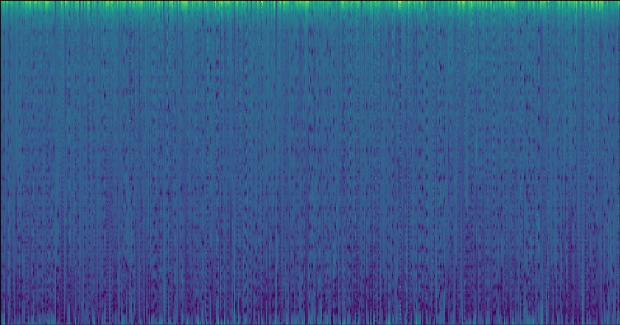
At this point, we can visualize the basis functions we’ve learned:
Each one-pixel-wide vertical slice of this image represents a single basis function. To encode a single frame of audio, we need to record its euclidean norm, and which of the 512 centroids, or basis functions, is closest in euclidean space to the frame we’re encoding.
In zounds in-browser interactive REPL, We can do an encode and decode pass for a particular piece of audio like so:
>>> kmeans = DctKMeans()
>>> doc = Document(_id='FlavioGaete22/TFS2_TVla09.wav')
>>> transform_result = kmeans.pipeline.transform(doc.mdct)
>>> recon_mdct = transform_result.inverse_transform()
>>> synth = zounds.MDCTSynthesizer()
>>> recon_audio = synth.synthesize(recon_mdct)
Then, we can listen back to some audio alongside the reconstructions from our encoder to subjectively evaluate its performance.
Monophonic Phrase
Problems with our encoder become apparent right away. The original sound is a high-pitched phrase with rich harmonics, but our reconstruction sounds like something out of an Atari game.
Original
Reconstruction
Broad-Band Synth
This synth sound has tons of texture and a very broad frequency range, but our reconstruction only captures the low frequencies, sounding muffled and garbled.
Original
Reconstruction
Drum Beat
This simple drumbeat has a bassy kick, and high, clicky hi-hat sounds. Our reconstruction recreates the kick drum, and not much else.
Original
Reconstruction
Cello
Here’s a short cello-like phrase. Our reconstruction ends up back in Atari-land.
Original
Reconstruction
Adding Log Amplitude
The original encodings sound pretty awful for a couple reasons:
- They tend to emphasize the single, dominant frequency in a frame, and ignore the rest
- They tend to over-emphasize lower frequencies
We actually tend to perceive amplitude on something like a logarithmic scale, meaning that while we’re able to perceive a huge range of sound pressure levels, our perception of those levels is compressed, or smooshed (a technical term) closer together.
This could explain why our basis functions just seem wrong at this point, and our reconstructions sound awful: the single loudest frequency dominates the euclidean distance calculation when we’re learning our basis functions.
We’ll try a new pipeline that attempts to compensate for this problem by using a log amplitude scale:
@zounds.simple_settings
class DctKmeansWithLogAmplitude(ff.BaseModel):
    """
    A pipeline that applies a logarithmic weighting to the magnitudes of the
    spectrum before learning centroids,
    """
    docs = ff.Feature(
            ff.IteratorNode,
            store=False)

    # randomize the order of the data
    shuffle = ff.NumpyFeature(
            zounds.ReservoirSampler,
            nsamples=1e6,
            needs=docs,
            store=True)

    log = ff.PickleFeature(
            zounds.Log,
            needs=shuffle,
            store=False)

    # give each frame unit norm, since we care about the shape of the spectrum
    # and not its magnitude
    unit_norm = ff.PickleFeature(
            zounds.UnitNorm,
            needs=log,
            store=False)

    # learn 512 centroids, or basis functions
    kmeans = ff.PickleFeature(
            zounds.KMeans,
            centroids=512,
            needs=unit_norm,
            store=False)

    # assemble the previous steps into a re-usable pipeline, which can perform
    # forward and backward transformations
    pipeline = ff.PickleFeature(
            zounds.PreprocessingPipeline,
            needs=(log, unit_norm, kmeans),
            store=True)
Now, our basis functions look like this:
Monophonic Phrase
When we revisit the monophonic phrase with our log-amplitude encoder, we still have something that probably belongs in a video game, but the relationship between frequencies sounds more natural, and there are audible harmonics.
Original
Reconstruction
Broad-Band Synth
Here, we lose a lot of the rhythmic separation between notes, but again, the spectrum sounds much more natural, and not entirely dominated by bass frequencies.
Original
Reconstruction
Drum Beat
Hey listen to that, the hi-hat is back!
Original
Reconstruction
Cello
We’re back to the 8-bit video game music to some degree, but the texture definitely sounds more cello-like.