Audio Query-By-Example via Unsupervised Embeddings
A couple of months ago, I gave a talk at the Austin Deep Learning Meetup about building Cochlea, a prototype audio similarity search engine. There was a lot to cover in an hour, some details were glossed over, and I’ve learned a few things since the talk, so I decided to write a blog post covering the process in a little more detail.
Motivations and First Steps
There are countless hours of audio out there on the internet, and much of it is either not indexed at all, or is searchable only via subjective, noisy and relatively low-bandwidth text descriptions and tags. What if it was possible to index all this audio data by perceptual similarity, allowing musicians and sound designers to navigate the data in an intuitive way, without depending on manual tagging?
The first challenge in building this kind of index is producing a representation of short audio segments that captures important perceptual qualities of the sound. This is, of course, subjective, and somewhat task-dependent (e.g., am I searching for audio with a similar timbre, or just the same pitch, or maybe a similar loudness envelope?), but in this case, we’d like to find some embedding space where elements are near one another if a human would likely assign the two sounds to the same class. For example, two segments of classical solo piano music should fall closer together in the space than a segment of solo classical piano music and a segment of rock music.
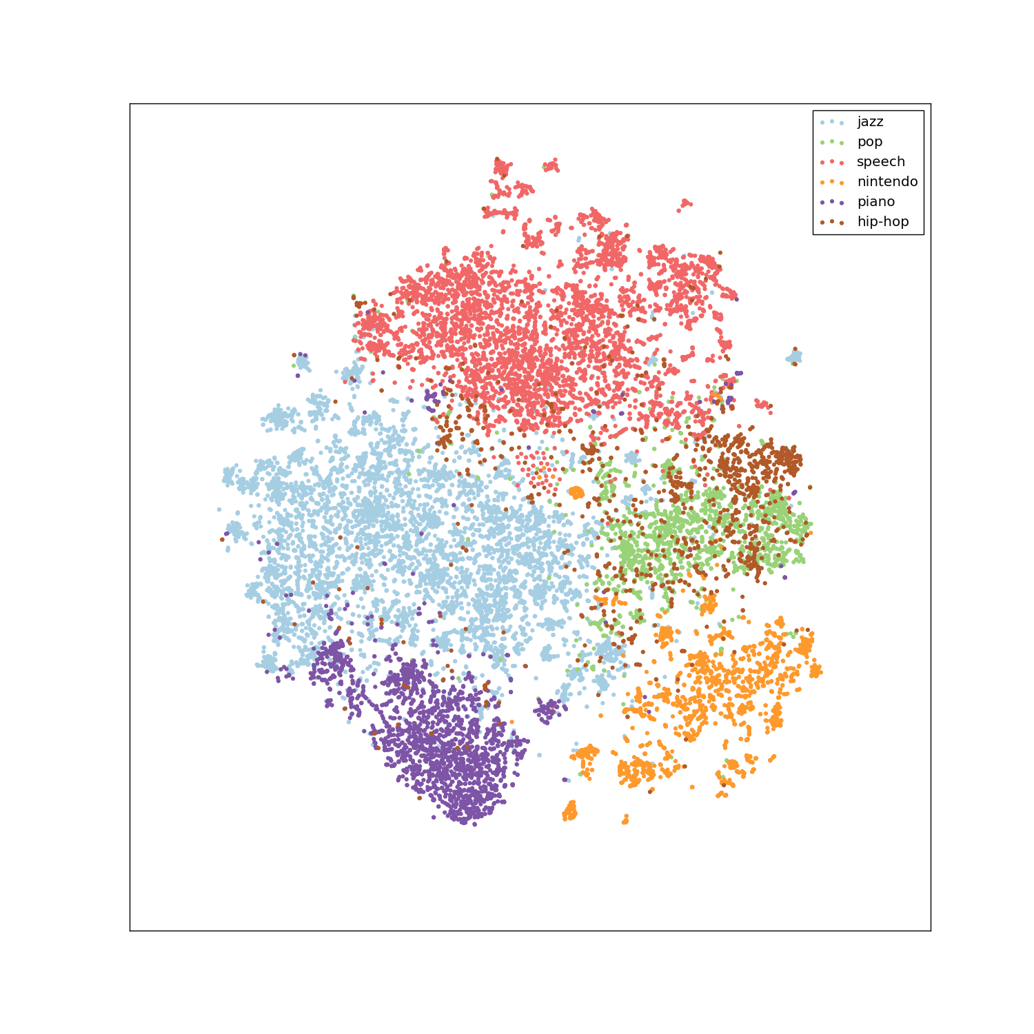
Above, you can see a t-SNE visualization of the 128-dimensional embeddings we end up learning in this experiment. What’s interesting here is that we’re plotting by tags or labels, but those won’t be used during training at all! We’ll train a neural network that separates audio classes fairly well in an unsupervised manner.
Unsupervised Learning of Semantic Audio Representations
There’s a great paper called Unsupervised Learning of Semantic Audio Representations from Dan Ellis’ research group at Google that develops the kind of representation we’re after by first noting a few things:
- certain types of transformations (e.g. pitch shifts and time dilation/compression) don’t typically change the general sound class
- sounds that are temporally proximal (occur near in time) tend to be assigned to the same sound class
- mixtures of sounds inherit the sound classes of the constituent elements
They leverage these observations to train a neural network that produces dense, 128-dimensional embeddings of short (approximately one second) spectrograms such that perceptually similar sounds have a low cosine distance, or small angle on the unit (hyper)sphere in an unsupervised fashion, without requiring a large, hand-labeled audio dataset to get started.
Deformations
First, to prove to ourselves that the observations are valid, we can apply the deformations to some audio and listen to ensure that some kind of perceptual similarity is maintained.
| Deformation | Audio |
|---|---|
| original | |
| pitch shift up | |
| pitch shift down | |
| time dilation | |
| time compression | |
| additive noise | |
| temporal proximity beginning | |
| temporal proximity end |
These all sound like they belong to the same, or a similar sound class, to my ears at least.
Triplet Loss
Getting a little more formal, we’d like to learn a function or mapping such that simple cosine distance in the target or embedding space corresponds to some of the highly complex geometric relationships between the anchor and deformed sounds represented in the audio we’ve just listened to.
For this experiment, that function, which we’ll call $g$, will take the form of a deep convolutional neural network with learn-able parameters:
\[g: \mathbb{R}^{F \times T} \rightarrow \mathbb{R}^{embedding\_dim}\]The original space is expressed as having dimensionality $F \times T$ because the input representation used in the paper is a spectrogram, with the $^F$ and $^T$ representing the frequency and time dimensions, respectively. We’ll go into more detail about how this representation will be computed in the next section.
Our dataset will consist of $N$ “triplets” of data:
\[\tau = \{ t_i\}_{i=1}^N\]Each triplet will look something like this:
\[t_i = (x_{a}^{(i)}, x_{p}^{(i)}, x_{n}^{(i)})\]and each member of the triplet will be a spectogram:
\[x_a^{(i)}, x_p^{(i)}, x_n^{(i)} \in \mathbb{R}^{F \times T}\]Each $x_a$ represents an anchor audio segment, each $x_p$ represents a positive example, i.e., the anchor with one of our audio deformations applied, or another audio segment that occurs near in time to the anchor, and each $x_n$ represents a negative example, which we’ll choose by picking any other audio segment from our dataset at random. Given a large enough dataset, our random strategy for choosing the negative example is probably fairly safe, but we will take some care to not accidentally choose negative examples that are actually more perceptually similar to the anchor than the positive example.
We’ll minimize a loss with respect to our network parameters that will try to push the anchor and positive examples closer together in our embedding space, while it also pushes our anchor and negative examples further apart, given some distance function $d$:
\[\mathcal{L}(\tau ) = \sum_{i=1}^{N}\left [ d(g(x_a^{(i)}), g(x_p^{(i)})) - d(g(x_a^{(i)}), g(x_n^{(i)})) + \delta \right]_+\]Our network’s job is to ensure that the distance $d$ from anchor to positive examples is less than the distance from anchor to negative examples by some positive margin $\delta$. The paper’s authors used squared l2 distance as their $d$:
\[d(a, b) = \left \| a - b \right \|_2^2\]While I used cosine distance:
\[d(a, b) = 1 - \frac{a \cdot b}{\left\| a \right\|_2 \left\| b \right\|_2}\]The $_+$ here indicates the hinge loss,
which really just means that our loss goes to zero if it’s less than this
margin $\delta$. As usual, since we can’t optimize this term over all $N$
triplets, we’ll optimize the learn-able parameters using minibatches of data.
Additionally, we’ll see later that because of the way we’re sampling these
triplets, our dataset is effectively unbounded.
Log-Scaled Mel Spectrograms
The paper’s authors compute their input spectrograms by:
- using short-time Fourier transforms
- discarding phase
- mapping the resulting linear-spaced frequency bins onto an approximately log-spaced Mel scale
- applying a logarithmic scaling to the magnitudes
This is a fairly standard pipeline for computing a perceptually-motivated audio representation. They go on to apply the various deformations mentioned above directly to this time-frequency representation. I was a little uneasy with this approach because:
- mapping onto the Mel scale is done after the fact, from linear-spaced frequency bins that don’t have the frequency resolution we’d like in lower frequency ranges and are needlessly precise in higher frequency ranges
- the representation isn’t invertible, as phase is discarded and many frequency bins in the higher ranges are averaged together, meaning that it’s impossible to know if the transformations actually sound plausible.
For this project, I decided to perform all deformations in the time domain, mostly to convince myself that all of them continued to sound plausible. I also opted to compute the time-frequency representation using a bank of log-spaced Morlet wavelets, so that perceptually-inspired frequency spacing and time/frequency resolution trade-offs could be accounted for from the outset, instead of being something of an afterthought. A subset of our bank of filters will look something like this:
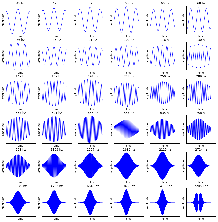
This filter bank can be thought of as a 1D convolutional layer with frozen parameters. Visualizing all the channels and weights of our convolutional filter bank at once yields something like this:
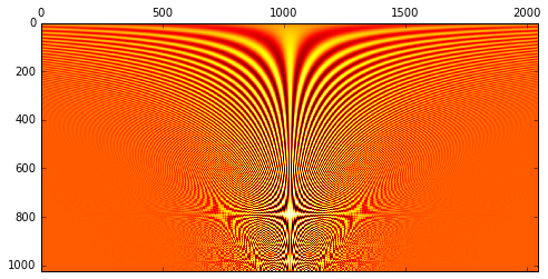
One nice side effect of this decision is that now the computation of the time-frequency transform is performed as part of our neural network, or as part of our function $g$, by a convolutional layer with frozen parameters, meaning that our input representation is now just $\mathbb{R}^T$, with $^T$ being the number of audio samples in each segment. While the filter bank is not included in the network’s learn-able parameters for this initial experiment, a learn-able time-frequency transform is an open possibility in future iterations of this work.
The time-frequency representations we compute will look something like this:

You can see the implementation of our
learn-able $g$ function here,
which uses the zounds.learn.FilterBank
module to compute the time frequency-representation before passing it on to a
stack of convolutional layers. Also, this jupyter notebook
offers a more in-depth exploration of the motivations behind using a bank of
log-spaced Morlet wavelets to compute our log-frequency representation.
Within-Batch Semi-Hard Negative Mining
The paper’s authors also use a technique called “within-batch, semi-hard negative” mining to make training batches as difficult as possible for the network. Since our loss encourages our learn-able function to widen the gap between the anchor-to-positive and anchor-to-negative embedding distances, we’d like to arrange our training data in such a way that that gap between embeddings is narrowed, forcing our network to work harder to push anchor and negative embeddings further apart, and anchor and positive embeddings closer together. Picking the hardest negative example for each anchor requires that we compute the distance from every anchor embedding to every negative embedding. This is obviously prohibitively slow to do with our entire dataset, and again, isn’t really possible due to the fact that we’re building batches on the fly, so we’ll instead do it only within each batch.
You can see the results of this process on several batches of size eight in the graph below. After re-assigning the negative examples, the new anchor-to-negative distances (in red) for each example tend to be closer to the anchor-to-positive distances (in blue) than the original anchor-to-negative distances (in green), while still maintaining a positive margin. It’s worth noting that the technique I’m using to re-assign the negative examples allows for the same negative example to be assigned to multiple triplets if it meets the criteria we set out above.

There’s a little more detail about the algorithm I used to perform within-batch semi-hard negative mining in this jupyter notebook.
Training Data
The paper’s authors used Google’s AudioSet for their training data, but I chose to pull together around 70 hours of sound and music from various sources on the internet, including:
While AudioSet is fantastic and enormous, my ultimate goal is to index audio on the internet in the same way Google that indexes documents, so I wanted to get some practice scraping audio and related metadata from disparate sources on the internet as a part of this work.
Training
Now that all the details are ironed out, training the network is fairly straightforward and follows this procedure:
- choose a minibatch of anchor examples at random
- either apply a deformation (e.g., time stretch or pitch shift) or choose segments that occur within ten seconds of each anchor to produce positive examples
- choose negative examples at random to complete the triplets
- use our network $g$ in its current state to compute embeddings for the anchor, positive, and negative examples
- perform within-batch semi-hard negative mining, re-assigning some or all of the negative embeddings to make each example in the batch “harder”, i.e., the loss greater
- compute triplet loss, calculate gradients via backpropagation, and update our network’s weights
Building an Index with Random Projections
Naively, if we’d like to use our new embedding space to support query-by-example, it means computing the distance between a query embedding and every other segment in our database! A brute-force distance computation over every embedding obviously won’t scale well, but thankfully there are plenty of techniques available for performing approximate K-nearest neighbors search over high-dimensional data in sub-linear time.
One such approach that gets us log-ish retrieval times builds a binary tree from every embedding in our dataset by choosing a random hyperplane for each node in the tree and bisecting that node’s data based on which side of the hyperplane each data point lies. Erik Bernhardsson took this basic approach while working on music recommendations at Spotify, along with some clever tricks to improve accuracy, and open-sourced his work as a library called Annoy (Approximate Nearest Neighbors Oh Yeah).
Here’s a visualization of a single hyperplane tree built from our learned embeddings:

The first trick introduced is simply to search both of a node’s subtrees when a query vector lies sufficiently close to that node’s hyperplane. The intuition here is that good candidate vectors that lie just on the other side of the hyperplane “fence” would be missed, despite the fact that they’re nearby.
The second trick is to build multiple trees. All of the trees can be searched in parallel by building a priority queue of nodes to search, where node priority is determined by how far the query vector lies from that node’s hyperplane. As we observed when discussing the first trick, hyperplanes that are far from the query vector are more likely to catch nearby candidates, so we’ll prefer those nodes, searching until we’ve reached some threshold of candidates we’d like to consider.
Finally, we perform a brute-force distance search over our pool of narrowed candidates, which is typically orders of magnitude smaller than our total index size.
In the graph below, you can look at the speed/accuracy tradeoffs we can make for our search using from one to 64 trees. Accuracy here (ranging from 0-1) on the x-axis is defined as the overlap with results from our brute-force source-of-truth search. There are other parameters that can be tweaked, such as our threshold for searching both paths for a given node, and the size of the candidate pool over which we’ll perform our final brute-force search, but this holds those parameters constant, only varying the number of trees we’re using. These timings are for searches over around 60 hours of audio.

It’s worth noting that these timings are based on a pure-Python/Numpy implementation of the algorithm that I wrote for learning purposes; timings from Annoy’s C++ implementation would likely look better.
Conclusion and Next Steps
We’re off to a pretty good start. We’ve now got:
- A way to learn a representation that captures perceptual similarity in an unsupervised way. The more data we can feed it, the better!
- A pretty fast way to search
There are some interesting avenues to explore going forward, however:
- Does vector arithmetic work for these embeddings just like it does for word
embeddings (i.e., the classic
king - man + woman = queenexample)? Can we find a piano and violin duet by adding their “solo” embeddings together? - Could these embeddings be used in audio synthesis as conditioning vectors for a WaveNet-like model or a conditional WaveGAN?
- Can we use these embeddings to predict tags for unlabelled audio for enhanced text search?
- Is it possible to further embed our representations in a much lower two or three-dimensional space, making the navigation of audio segments visual and intuitive (our t-SNE visualization above points to “yes”)?
Resources
- You can find slides from the original talk here, and watch a video of it on YouTube.
- All the code for this experiment is on GitHub
- Unsupervised Learning of Semantic Audio Representations is the paper on which this experiment is based
- There’s a good blog post where Annoy’s author explains it in detail and an talk that covers the same material on YouTube.