Building a Timbre-Based Similarity Search
For quite some time, I’ve been fascinated with the idea of indexing large audio corpora, based on some perceptual similarity metric. This means that it isn’t necessary for some human to listen to and tag each audio sample manually. Searches are by example (rather like the “search by image” feature that you’ve probably encountered), and it’s possible to explore “neighborhoods” of similar sounds.
Prototyping these kinds of systems can be cumbersome and time-consuming. I’ve built enough of them from scratch to know that I spend the majority of my time not on the idea itself, but rather on the mundane, but totally necessary details of:
- how to ingest lots of audio for a test bed
- how to extract common audio features
- how to use unsupervised learning to find good representations of the audio
- how to index and search those representations
- how and where to persist all of this data
Zounds was built with a mind to solving all of these common problems so that you have more time to focus on your idea, and spend less on bookkeeping.
The Idea
We’d like to be able to find similar groups of sounds in a large corpus, based on their timbre.
tim·bre
the character or quality of a musical sound or voice as distinct from its pitch and intensity.
Here’s a group of sounds with similar timbre, from a search interface built using zounds.
In order to do that, we’ll be working from this example from the zounds repository, and building a very simple, timbre-based similarity search. Once you’ve read through this post, you shouldn’t need to write a single line of code; just run this example from the zounds repository, and it will run through each of the steps described below.
We’ll be glossing over a lot of details; the goal is to get a high-level idea of what it takes to build such a search. We’ll explore some of the building blocks in much more detail in later posts.
Defining our Baseline Features
Given that we want to group audio roughly by timbre (which is admittedly a very subjective thing), we’ll need to transform audio in such a way that we achieve some translation invariance in the frequency domain. Put another way, we’d like to understand something about the “shape” of the audio spectrum, or the relationships therein, ignoring the exact positions or frequencies of these shapes.
One of the most common ways to achieve this is to use a feature like MFCC, or Mel-frequency cepstral coefficients. Roughly speaking, this is a spectrum of a spectrum, discarding phase, so we get an idea of what kinds of intervals, or relationships are present between dominant frequencies in the spectrum.
The first step will be to define a class WithTimbre that will first extract bark bands from the short-time fourier transform frames, and then compute the cepstral coefficients of those frames.
import featureflow as ff
import zounds

class Settings(ff.PersistenceSettings):
    id_provider = ff.UuidProvider()
    key_builder = ff.StringDelimitedKeyBuilder()
    database = ff.LmdbDatabase(path='timbre', key_builder=key_builder)


windowing = zounds.HalfLapped()
STFT = zounds.stft(resample_to=zounds.SR22050(), wscheme=windowing)


class WithTimbre(STFT, Settings):
    bark = zounds.ConstantRateTimeSeriesFeature(
            zounds.BarkBands,
            needs=STFT.fft,
            store=True)

    bfcc = zounds.ConstantRateTimeSeriesFeature(
            zounds.BFCC,
            needs=bark,
            store=True)
Now calling…
>>> _id = WithTimbre.process(meta=some_file_like_object_or_url)
…will extract the bark and bfcc features and persist them in an LMDB database on your local filesystem.
For a cello sound like this:
Calling…
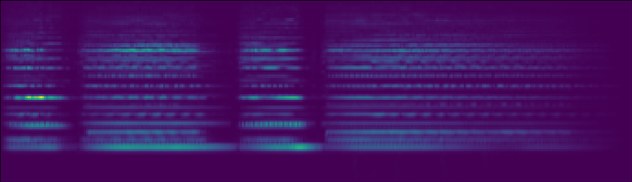
>>> WithTimbre(_id).bark
…will return a ConstantRateTimeSeries instance, which is really just a subclass of numpy.ndarray that knows about the frequency and duration of its samples. It’ll look like this, for an audio file containing a short snippet of a cello playing:
Then, calling…
>>> WithTimbre(_id).bfcc
…will return another ConstantRateTimeSeries that looks something like this, for the same cello sound:

Getting a Corpus of Data
There a tons of great places to find free audio samples online, but I happened upon this page, hosted by the One Laptop Per Child organization. After browsing the sample sets available there, I decided that this set looked like it had enough samples, and enough variety to make this search interesting.
We’re going to download this file, and use the WithTimbre class we defined above to extract bark-frequency cepstral coefficients by streaming each audio file from the zip archive:
# Download the zip archive
url = 'https://archive.org/download/FlavioGaete/FlavioGaete22.zip'
filename = os.path.split(urlparse(url).path)[-1]

resp = requests.get(url, stream=True)

print 'Downloading {url} -> {filename}...'.format(**locals())

with open(filename, 'wb') as f:
    for chunk in resp.iter_content(chunk_size=4096):
        f.write(chunk)

# stream all the audio files from the zip archive
print 'Processing Audio...'
for zf in ff.iter_zip(filename):
    if '._' in zf.filename:
        continue
    print zf.filename
    WithTimbre.process(meta=zf)
Notice the call to WithTimbre.process(meta=zf) in the very last line there.
Learning a Good Representation
Now that we’ve processed all that audio, and persisted the extracted features to disk, we’d like to learn a representation of the features that is binary, making it possible to pack those features into bitarrays, and perform a brute-force, but fast bitwise hamming distance computation against every example in our dataset.
We’ll start by doing K-Means clustering on our WithTimbre.bfcc feature. First, we’ll define the pipeline for extracting a model from our dataset:
@zounds.simple_settings
class BfccKmeans(ff.BaseModel):
    docs = ff.Feature(
            ff.IteratorNode,
            store=False)

    shuffle = ff.NumpyFeature(
            zounds.ReservoirSampler,
            nsamples=1e6,
            needs=docs,
            store=True)

    unitnorm = ff.PickleFeature(
            zounds.UnitNorm,
            needs=shuffle,
            store=False)

    kmeans = ff.PickleFeature(
            zounds.KMeans,
            centroids=128,
            needs=unitnorm,
            store=False)

    pipeline = ff.PickleFeature(
            zounds.PreprocessingPipeline,
            needs=(unitnorm, kmeans),
            store=True)
This pipeline will:
- randomly sample from, and shuffle the dataset it receives
- give each example unit norm, because again, we’re interested in the shape of these examples, and not their magnitude
- Learn 128 means from the data
- Produce a pipeline that is now capable of transforming our
WithTimbre.bfccfeature into a one-hot encoding: a 128-dimensional vector with a single non-zero entry
To learn and persist our model, we just need to pass BfccKmeans an iterator over the examples we’d like it to learn from:
>>> BfccKmeans.process(docs=(wt.bfcc for wt in WithTimbre))
Building an Index
Now that we’ve learned a good representation of our WithTimbre.bfcc feature, we’d like to store that encoding. Additionally, we know our choice of feature gives us translation invariance in the frequency domain, but we’d also like to introduce some invariance in the time domain, so in addition to storing our one-hot encoding, we’ll also pool the feature together over short spans of time, so that, given our 128-dimensional one-hot encoding, pooled over say, 30 frames, we’d have a new 128-dimensional binary vector with at most 30 “on” entries, in the case where each of the thirty frames has a different code.
Concretely, for the same cello sound from above, we’d like to see our encoding looking something like this:
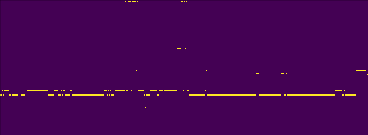
And we’d like to see the pooled version looking something like this:

To achieve this, we’ll define a new class, derived from our original WithTimbre class, that adds these new features:
class WithCodes(WithTimbre):
    bfcc_kmeans = zounds.ConstantRateTimeSeriesFeature(
            zounds.Learned,
            learned=BfccKmeans(),
            needs=WithTimbre.bfcc,
            store=True)

    sliding_bfcc_kmeans = zounds.ConstantRateTimeSeriesFeature(
            zounds.SlidingWindow,
            needs=bfcc_kmeans,
            wscheme=windowing * zounds.Stride(frequency=30, duration=30),
            store=False)

    bfcc_kmeans_pooled = zounds.ConstantRateTimeSeriesFeature(
            zounds.Max,
            needs=sliding_bfcc_kmeans,
            axis=1,
            store=True)
It’s interesting to note that these new stored features we’ve introduce will be computed lazily, on-demand. The first time I do something like:
doc = WithCodes(_id)
print doc.bfcc_kmeans_pooled
Both the WithCodes.bfcc_kmeans and WithCodes.bfcc_kmeans_pooled features will be computed and stored (the former will be computed because the latter depends upon it).
With that in mind, all we have to do now is to define and build our index over the WithCodes.bfcc_kmeans_pooled feature. The encodings we need will be computed and stored on-demand in the course of building the index.
BaseIndex = zounds.hamming_index(WithCodes, WithCodes.bfcc_kmeans_pooled)

@zounds.simple_settings
class BfccKmeansIndex(BaseIndex):
    pass

# build the index
BfccKmeansIndex.build()

# get an instance of the index
index = BfccKmeansIndex()
Searching the Data
Finally, if we’d like to get an idea of whether we’ve sucessfully built an index that finds perceptually similar sounds, we can play around in the in-browser interactive repl. There’s a random_search method on the index we’ve built that chooses a random sample from the already-indexed data as a query, and then returns the n most similar or relavent results.
>>> index.random_search()
Once again, here’s an example group of similar results, from a search interface built using zounds.