The last couple of posts have been all about audio analysis and search but in this one, I’ll return to some work that gets me a little closer to my ultimate goal, which is building synthesizers with high-level parameters, allowing the production of audio ranging from convincingly-real renderings of traditional acoustic instruments to novel synthetic textures and sounds.

There’s clearly a lot of value in symbolic (usually MIDI-based) approaches to music generation but I feel there’s incredible promise and flexibility in producing audio directly. Some incredibly moving sequences of sound are also very difficult to score, and not every valid or valuable piece of music can be expressed as a collection of discrete notes or events.

All of the code for this, and future experiments involving music synthesis, can be found in this GitHub repo.

A Break in the Case

I had already been exploring the use of generative adversarial networks to produce very short and noisy snippets of Bach piano music when I read the WaveGAN paper, which was the first published application of GANs to raw audio that I’m aware of. This was a very exciting and insightful paper, but I got really excited last year when I read a pair of papers that had something very cool in common.

Those were:

• MelGAN: Generative Adversarial Networks for Conditional Waveform Synthesis
• High Fidelity Speech Synthesis with Adversarial Networks

Both papers focused primarily on speech (the MelGAN paper included piano samples as an aside) but the interesting feature they shared is that they were both training strongly-conditioned GANs using low-frequency audio features as input to the generator, which would then output high-frequency raw audio samples.

What really excited me about these papers is that they seemed to lay the foundation for a very flexible two-stage music synthesis pipeline. At its simplest, two trained networks would be required:

1. A strongly-conditioned generator that can produce convincing audio from low-frequency features
2. Another network, unconditioned or perhaps conditioned on yet higher-level features, that could produce plausible sequences of these low-frequency features

This post will focus on the first stage in that pipeline, with a subsequent post covering the generation of novel musical sequences.

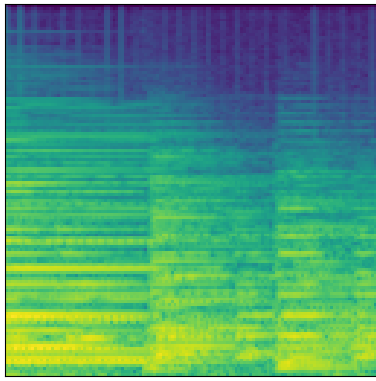
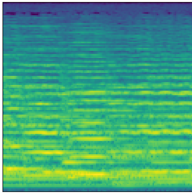
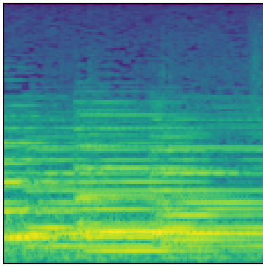
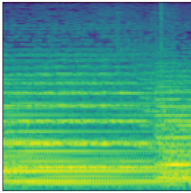
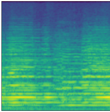
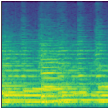
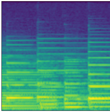
Since my focus is music, I chose to use the MusicNet dataset, which consists of around 34 hours of classical music recordings. As my low-frequency conditioning feature, I chose to use 128-bin Mel-frequency spectrograms. Here are a couple examples of audio from the dataset, alongside the accompanying low-frequency Mel spectrograms:

First Attempt: Assessing the MelGAN for the Task

The first and most obvious approach would be to use the architecture described in the MelGAN paper, mostly as-is, and assess its performance on the task of producing musical signals.

The MelGAN paper focuses primarily on speech but you can hear some examples of both speech and music generation from the model on this page.

I had reason to be skeptical about the architecture’s performance on fairly diverse musical signals based on the piano examples included in that page, but decided starting with the MelGAN architecture would serve as a good baseline.

The MelGAN paper uses a single generator that makes use of dilated convolutions to greatly expand the receptive field of its layers, as well as multiple discriminators that operate at a few different time scales/sampling rates. Notably, the discriminators don’t just produce a single judgement per input example; they produce multiple, overlapping judgements in the time domain.

The generator is fully convolutional, meaning that it makes no assumptions about the input or output time dimension. This is a handy feature in a vocoder, since we can pass it a spectrogram of virtually any length at inference time.
During training, windows of 8192 samples at 22050hz (about a third of a second) are used.

In the usual GAN setting, the generator is only trying to minimize or maximize some scalar value that the discriminator computes to indicate how close to the real training data the synthetic data lies. The MelGAN paper adds to this a feature-matching loss, in which the generator tries to minimize the L1 distance between discriminator feature maps, or internal activations, for synthetic and real data.

It’s interesting to note that the discriminator does not have access to the conditioning information in the original MelGAN formulation; it is purely computing the distance between real and fake examples. When the generator loss is computed, discriminator feature maps are compared within the same batch, so that feature maps from real audio samples are being compared against feature maps from audio generated based on spectrograms derived from that same audio.

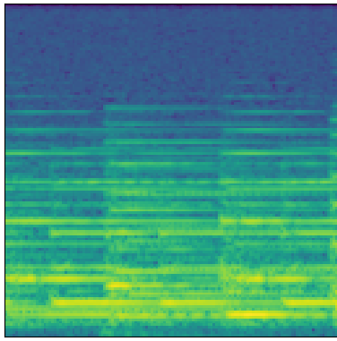
As you can hear, the generator captured the overall structure of the audio fairly well after around 12 hours of training, but produced reproductions that were somewhat metallic and noisy:

Real

Generated

Real

Generated

More generated samples can be heard here.

An Alternate Architecture Geared Toward Music

After evaluating the original MelGAN architecture’s performance on MusicNet, and trying quite a few alternative approaches, I settled on the some modifications to the original experiment that resulted in more pleasing/musical audio.

Over the course of several experiments, I found that giving the discriminator access to the conditioning data generally accelerated training and made for better end results. I also found that building some strong priors into both the generator and discriminator architectures seemed to help with producing crisper and more pleasant audio.

Before we dive in, code for the top-level parameters of this experiment can be found here.

A Conditioned Discriminator

First, several experiments seemed to indicate that allowing the discriminator access to the conditioning spectrograms accelerated training and made for better end results. It’d be worth an ablation study with my best-performing generator and discriminator to find out if this impression is true, but I haven’t yet performed one.

Strong Audio Priors

While one of the promises of deep learning is models that learn from scratch, there may be cases where aspects of human perception are difficult or impossible to learn without some strong guidance. With that in mind, and in hopes of accelerating training, my generator and discriminator architectures have in-built priors based on two facts:

• Musical audio contains information at many different time-scales
• Our perception of sound depends a great deal on a decomposition of audio into many frequency bands by the cochlea

Multi-Scale Generator and Discriminator

To address the problem of information at vastly different time scales, I saw an opportunity to try a multi-scale analysis and synthesis idea that mirrors multi-resolution wavelet transforms or the Non-stationary Gabor Transform.

In most raw audio-producing neural network architectures I’ve encountered thus far, all audio and thus all frequency bands are produced at the same sampling rate. I wanted to try an architecture where groups of frequency bands were produced at an appropriate sampling rate, such that low frequency bands could be faithfully rendered with significantly fewer samples and only up-sampled at the last possible moment. My hunch was that over-sampled filters producing lower frequencies were likely to produce a lot of artifacts.

More concretely, at 22050hz, we might represent one second of audio with the following five bands or channels:

N samples	Start Hz	End Hz
1378	0	689
2756	689	1378
5512	1378	2756
11025	2756	5512
22050	5512	11025

So, we might decompose the following audio samples at 22050hz…

…into the following five bands

0hz - 689hz

689hz - 1378hz

1378hz - 2756hz

2756hz - 5512hz

5512hz - 11025hz

For this experiment, the top-level generator was composed of five distinct frequency band generators that produced audio on each of the five time scales represented above. Each sub-generator is conditioned on the same input spectrogram.

Similarly, the discriminator is composed of five distinct frequency band discriminators that analyze audio on each of the five time scales represented above. Each of these also have access to the conditioning spectrogram.

Frozen Filter Bank Layers

To mimic the decomposition of audio into constituent frequency bands by the cochlea, each sub-generator and sub-discriminator includes a frozen layer (i.e., a layer with no learn-able parameters) representing a bank of finite impulse response filters. This is similar to an approach used in the paper Speaker Recognition from Raw Waveform with SincNet where the first layer of a speech recognition model is initialized as a bank of finite impulse response filters, parameterized by the filters’ center frequencies and bandwidths.

In this case, the discriminator for each time scale will have a frozen first layer initialized as a linear-spaced filter bank spanning the frequency interval [nyquist / 2, nyquist] except for the lowest-frequency time scale, whose filter bank will span [0, nyquist].

The generator for each time scale will also include one of these frozen filter bank layers, this time as its last layer. The generator will produce audio by performing a transposed convolution with this layer as its last step, essentially summing together the excitations from each filter bank channel.

During training, the discriminator views audio as N distinct bands at different time scales and the generator produces this same representation. Only during inference does each generated band need to be resampled to the desired sample rate (22050hz in our case) and summed together to produce the final output.

Conditioned Audio Examples

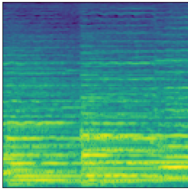
Now that we’ve covered the modifications to the generator and discriminator architectures, let’s listen to some samples generated by the new model:

Real

Generated

Real

Generated

Real

Generated

Real

Generated

Real

Generated

Real

Generated

These samples tend to be less noisy and metallic-sounding than those produced with the baseline MelGAN architecture. To my ear, they are more faithful to the originals, and more musically pleasant. They aren’t without their problems, however. There are some significant phase issues, possibly due to the fact that each generator band is produced independently. The model also seems to have trouble faithfully reproducing lower frequencies which I find somewhat puzzling and surprising.

You can hear more generated examples here.

Future Work

Overall, the results are promising and lay the groundwork for a first step in our two-stage music synthesis pipeline. Next steps will include:

• Beginning to work on contioned or unconditioned Mel spectrogram generation using this trained model as the spectrogram-to-audio vocoder
• Exploring strategies for mitigating phase issues in this model
• Exploring strategies for reproducing low frequencies more faithfully
• Performing a more principled comparison of the original MelGAN model with this one, including analysis of parameter counts, audio generation performance and a more careful side-by-side analysis of generated samples