Sparse Interpretable Audio Model
This post covers a model I’ve recently developed that encodes audio as a high-dimensional and sparse tensor, inspired by algorithms such as matching pursuit and dictionary learning.
Its decoder borrows techniques such as waveguide synthesis and convolution-based reverb to pre-load inductive biases about the physics of sound into the model, hopefully allowing it to spend capacity elsewhere.
The goal is to arrive at a sparse, interpretable,
and hopefully easy-to-manipulate representation of musical sound. All of the model training and inference
code can be found in the matching-pursuit github repository,
which has become my home-base for audio machine learning research.
The current set of experiments is performed using the MusicNet dataset.
⚠️ This post contains sounds that may be loud. Please be sure to start your headphones or speakers at a lower volume to avoid unpleasant surprises!
Motivations
I’ve formed several hunches/intuitions in my recent years working on machine learning models for audio synthesis that all find expression in the work being covering today.
Frame-Based Representations Are Limited
Almost all codecs and machine learning models that perform audio analysis and/or synthesis are frame-based; they chop audio up into generally fixed-size frames, without much regard for the content, encode each framem and represent audio as a sequence of these encodings.
The model discussed today takes some baby-steps away from a frame-based representation, and toward something that might be derived using matching pursuit or dictionary learning.
While a sequence of encoded frames may reproduce sound very faithfully, it is not easily interpretable; each frame is a mixture of physical or musical events that have happened before that moment, and continue to reverberate.
My sense is that a high-dimensional and very sparse representation maps more closely onto the way we think about sound, especially musical audio.
Audio Synthesis Models Must Learn Physics
While there are certainly classes of audio where the laws of physics are unimportant (synthesized sounds/music), those laws are integral to the sounds made by acoustic instruments, and even many synthesized instruments simply aim to mimic these sounds.
Do audio models waste capacity learning some of the invariant laws of sound from scratch? Could it be advantageous to bake some inductive biases around the physics of sound into the model from the outset, so that it can instead focus on understanding and extracting higher-level “events” from a given piece of audio?
Synthesis techniques such as waveguide synthesis and the use of long convolution kernels to model material transfer functions and room impulse responses suggest a different direction that might be fundamentally better (for audio) than the classic upsample-then-convolve-with-short-kernel approaches that have dominated both image and audio generation to-date.
Quick Tour
Before diving into the details, it might be good to get an intuitive feel for what the high-level components of the model are doing. We grab a random segment of audio from the MusicNet dataset…
from conjure import audio_conjure

@audio_conjure(conjure_storage)
def get_audio(identifier):
    from data.audioiter import AudioIterator
    from util import playable
    import zounds

    stream = AudioIterator(
        1,
        2**15,
        zounds.SR22050(),
        normalize=True,
        overfit=False,
        step_size=1,
        pattern='*.wav')
    chunk = next(iter(stream))
    chunk = chunk.to('cpu').view(1, 1, stream.n_samples)
    audio = playable(chunk, stream.samplerate)
    bio = audio.encode()
    return bio.read()

example_6 = get_audio('example_7c')
_ = get_audio.meta('example_7c')
You can click on the waveform to play the sound.
The Encoding
The network encodes the audio, and we end up with something like this.
⚠️ Because the representation is very high-dimensional,
(4096, 128)to be exact, we downsample for easier viewing
from conjure import numpy_conjure, SupportedContentType

@numpy_conjure(
    conjure_storage,
    content_type=SupportedContentType.Spectrogram.value)
def get_encoding(identifier):
    from models.resonance import model
    import zounds
    from io import BytesIO
    import torch
    from torch.nn import functional as F

    n_samples = 2**15
    bio = BytesIO(get_audio(identifier))
    chunk = torch.from_numpy(zounds.AudioSamples.from_file(bio)).float()
    chunk = chunk[...,:n_samples].view(1, 1, n_samples)

    encoded = model.sparse_encode(chunk)

    # downsample for easier viewing
    encoded = encoded[:, None, :, :]
    encoded = F.max_pool2d(encoded, (8, 8), (8, 8))
    encoded = encoded.view(1, *encoded.shape[2:])
    encoded = encoded[0].T
    return encoded.data.cpu().numpy()

encoding_1 = get_encoding('example_7c')
_ = get_encoding.meta('example_7c')
The dark-blue portions represent zeros, and the yellow-orange portions represent events.
Reconstructed Audio
We can also perform a full pass through the network, both encoding and decoding. The reconstructions don’t sound amazing, but are clearly the same musical sequence as the original.
from conjure import audio_conjure

@audio_conjure(conjure_storage)
def reconstruct_audio(identifier):
    from models.resonance import model
    from util import playable
    from modules.normalization import max_norm
    import torch
    import zounds
    from io import BytesIO

    n_samples = 2**15
    bio = BytesIO(get_audio(identifier))
    chunk = torch.from_numpy(zounds.AudioSamples.from_file(bio)).float()
    chunk = chunk[...,:n_samples].view(1, 1, n_samples)
    recon, _, _ = model.forward(chunk)
    recon = torch.sum(recon, dim=1, keepdim=True)
    recon = max_norm(recon)
    recon = playable(recon, zounds.SR22050())
    encoded = recon.encode()
    return encoded.read()

result = reconstruct_audio('example_7c')
_ = reconstruct_audio.meta('example_7c')
Another Reconstruction Example
original:
result = get_audio('example_8c')
_ = get_audio.meta('example_8c')
reconstruction:
result = reconstruct_audio('example_8c')
_ = reconstruct_audio.meta('example_8c')
Model and Training Details
The model’s encoder portion is fairly standard and uninteresting, while the decoder includes some novel features. Once again, code for the experiment can be found on github.
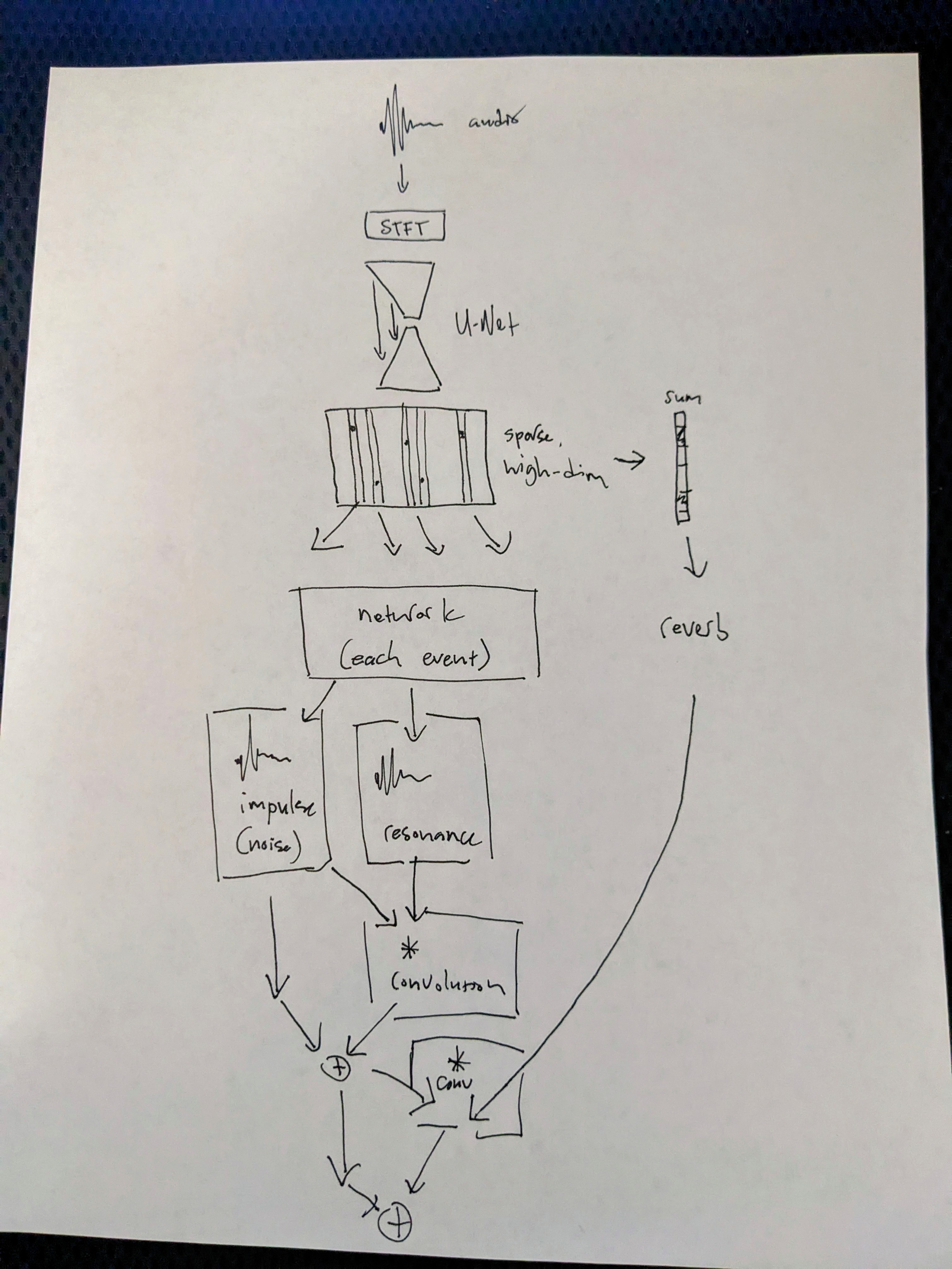
Encoder
Starting with 32768 samples at 22050 hz, or about 1.5 seconds of audio, we first perform a short-time fourier transform
with a window size of 2048 samples and a step size of 256 samples. This means that we begin with a representation of shape (batch, 1024, 128), where 1024
is the number of FFT coefficients and 128 the number of frames.
The spectrogram is then processed by a U-Net architecture with skip connections.
Finally, the reprsentation is projected into a high-dimensional space and sparsified by choosing the N top-k elements in the (batch, 4096, 128) tensor.
⚠️ The astute reader will notice that we’re working with the very frame-based representation we earlier warned against. There are still steps that need to be taken to fully free ourselves from the fixed-size grid.
Decoder
Beginning with our highly-sparse (batch, 4096, 128) representation, we “break apart” this tensor into N one-hot vectors. The current
experiment sets N = 64.
Put another way, we now have N or 64 one-hot vectors, ideally representing “events” for each element in the batch of examples. Next, we embed these high-dimensional one-hot vectors into lower-dimensional, dense vectors, and generate the audio for each event
independently from there.
First, we generate an impulse, which amounts to band-limited noise, representing the attack, breath, or some other injection of energy into a system.
Next we create a linear combination of a number of pre-generated resonance patterns, which amount to four different waveforms (sine, square, sawtooth, triangle) sampled at many different frequencies within the range of fundamental frequencies for most acoustic instruments, in this case, from 40 hz to 4000 hz. This represents the transfer function or impulse response of whatever system, or instrument, the impulse’s energy is injected into.
We also choose a decay value, which determines the envelope of the resonance and apply the envelope to the resonance we’ve generated.
Each impulse and resonance are then convolved to produce a single event.
The (batch, 4096, 128) encoding is also summed along its time-axis, such that it becomes (batch, 4096), and is then embedded into
a lower-dimensional, dense vector. This vector is passed to a sub-network which chooses a linear combination of impulse responses for
convolution-based reverb. Each event is also convolved with this room response kernel.
We end with a tensor of shape (batch, n_events, 32768), with each channel along the n_events dimension representing
Training
Instead of using MSE loss, each “event channel” loss is computed independently. There’s much more work to do to both refine this approach and understand better why it helps, but it does seem to encourage events to cover independent/orthogonal parts of the time-frequency plane. The model used to produce the encodings and audio in this post was trained for about 24 hours.
Random Generation
Finally, we can understand the model a little better (and have some fun) by generating random sparse tensors and listening to the results.
from conjure import audio_conjure

encoding_1 = get_encoding('example_7c')

@audio_conjure(conjure_storage)
def random_generation(identifier):
    import torch
    from models.resonance import model
    from modules import sparsify2
    from util import playable
    import zounds
    from torch.nn import functional as F

    n_samples = 2**15
    encoding = torch.zeros(1, 4096, 128).normal_(encoding_1.mean(), encoding_1.std())
    encoded, packed, one_hot = sparsify2(encoding, n_to_keep=64)
    audio, _ = model.generate(encoded, one_hot, packed)
    audio = torch.sum(audio, dim=1, keepdim=True)
    audio = playable(audio, zounds.SR22050())[..., :n_samples]
    bio = audio.encode()
    return bio.read()

result = random_generation('random_1d')
_ = random_generation.meta('random_1d')
Another random generation result:
result = random_generation('random_3d')
_ = random_generation.meta('random_3d')
Next Steps
- A single, low-dimensional and dense “context” vector for each audio segment might allow similar sparse vectors to represent related musical sequences played on different instruments, or in different rooms
- The “physical model” I’ve developed is very rudimentary. More study into existing physical modelling techniques might produce a far superior model
Thanks for Reading!
If you’d like to cite this article
@misc{vinyard2023audio,
  author = {Vinyard, John},
  title = {Sparse Interpetable Audio},
  url = {https://JohnVinyard.github.io/machine-learning/2023/11/15/sparse-physical-model.html},
  year = {2023}
}